Data Structures and Algorithms

By: Mohammad AbouElSherbini

Think 💡

(How does Google search or Youtube work?)

Agenda

Day 1
- Complexity analysis
- Divide and conquer
- Searching algorithms
- Sorting algorithms
Day 2
- Array
- LinkedList
- Stack
- Queue
Day 3
- Graph
- Tree
- BFS
- DFS
Day 4
- Set
- Map
- Heap / Priority Queue
Day 5
- Two pointers
- Sliding window
- Prefix sum
- Frequency array/map

Visualizations

Intro

How computers work

General purpose computers consist of 2 main components:

Hardware components: physical electronics that include CPU, GPU, RAM, etc..
Software components: instructions to these electronics which conveyed in a user friendly way by means of programing languages

With the evolution of electronic circuits it became easier to make a general purpose device that can change it’s functionality without having to change the hardware. but surely at the cost of less optimizations to each functionality.

So it’s very important to learn how to make good use of the instructions provided by the hardware.

Why learn

Problem Solving

Critical Thinking: Enhances logical reasoning and breaking down complex problems.
Adaptability: Prepares you for varied challenges.
Foundation: Essential for advanced computer science topics.

Data Structures

Efficient Data Management: Organize and manage data effectively.
Performance Optimization: Optimize for specific operations (e.g., search, insert).
Trade-offs: Choose the best structure for a problem.

Algorithms

Systematic Methods: Provide structured problem-solving techniques.
Efficiency: Write efficient and scalable code.
Innovation: Explore new problem-solving approaches.

Practical Application

Real-world Problems: Solve practical issues like network routing and data encryption.
Software Development: Write clean, efficient, and maintainable code.
Coding Interviews: Essential for technical job interviews.

What makes a good software

Software Engineering is a disciplined approach to the design, production, and maintenance of computer programs that are developed on time and within cost estimates, and utilizing tools that help to manage the size and complexity of the resulting software products.

Goals

Works (that is, accomplishes its intended function)
Can be read and understood
Can be modified if necessary without much effort
Is completed on time and within its budget.

Complexity analysis

Comparison of Algorithms:

Correctness: judged by how close you are to the answer or how many you got right
Runtime: judged by how long your code takes to run
Memory: judged by how much space your code needs

Analysis of Algorithms

Worst Case Analysis (Usually done): by calculating the upper bound(worst) of usages. annotated by Big O notations
Average Case Analysis (Sometimes done): by calculating the average of usages. annotated by Big Theta (Θ) notations
Best Case Analysis (Never done): by calculating the lower bounds(best) of usages. annotated by Big Omega (Ω) notations

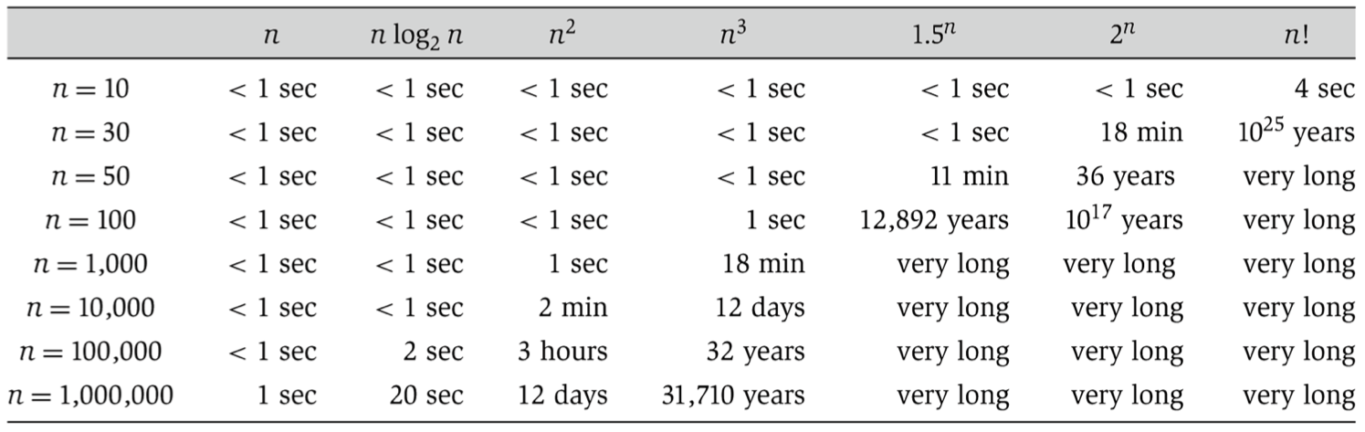
Estimating the Analysis

A simple way to get Big O notation of an expression is to drop low order terms and ignore leading constants (Why?). For example, consider the following expression.

3$n^3$ + 6$n^2$ + 6000 = O($n^3$)

Analysis comparison

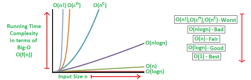
The common levels in order from best to worst:

0($1$): constant
O($log_2(n)$): logarithmic
O($n$): linear
O($n^2$): quadratic
O($n^3$): cubic
O($2^n$): exponential
O($n!$): factorial

Algorithms

Divide and conquer

Idea: used to solve problems by dividing the main problem into subproblems, solving them individually and then merging them to find solution to the original problem
Usual Complexity:
- Time: O($nlog_2(n)$)
- Space: O($n$)

Search Algorithms

Used to find one or more elements from a dataset.

We can achieve this using a linear search O(n) but with some extra information about the dataset we can further optimize the process

Examples:

Linear Search (Sequential Search): Works on random data, O($n$)
Binary Search: Works on sorted data, O($log_2(n)$)
Exponential Search: Works on sorted data, O($log_2(n)$)
Ternary Search: Works on sorted data, O($log_3(n)$)
Interpolation Search: Works on sorted data, good on uniform data but otherwise O($n$)

Linear search (Sequential Search)

Idea: iterate through the data one by one until you reach goal or dataset end
Complexity:
- Time: O($n$)
- Space: O($1$)

int search(int arr[], int N, int x) {
    for (int i = 0; i < N; i++)
        if (arr[i] == x)
            return i;
    return -1;
}

Binary search

Assumption: dataset is sorted
Idea: apply divide and conquer technique by dividing dataset into 2 segments, then checking the middle element to determine which segment to keep and which to discard, then repeat until you reach goal or dataset end
Complexity:
- Time: O($log_2(n)$)
- Space: O($1$)

Iterative:

int binarySearch(int arr[], int low, int high, int x) {
    while (low <= high) {
        int mid = low + (high - low) / 2;

        // Check if x is present at mid
        if (arr[mid] == x)
            return mid;

        // If x is smaller, ignore right half
        if (arr[mid] > x)
            high = mid - 1;

        // If x is greater, ignore left half
        else
            low = mid + 1;
    }

    // If we reach here, then element was not present
    return -1;
}

Recursive:

int binarySearch(int arr[], int low, int high, int x) {
    if (high < low) return -1; 
    
	int mid = low + (high - low) / 2;

	// Check if x is present at mid
	if (arr[mid] == x)
		return mid;

	// If x is smaller, ignore right half
	if (arr[mid] > x)
		return binarySearch(arr, low, mid - 1, x);

	// If x is greater, ignore left half
	return binarySearch(arr, mid + 1, high, x);
    
}

Labs

Implement Sequential Search & Binary Search on array of integers & cstrings (4 total)
69. Sqrt(x)
441. Arranging Coins

Sort Algorithms

Used to organize a dataset in a certain order.

There are many Algorithms to achieve this but with varying complexities like:

Selection Sort: O($n^2$)
Bubble Sort: O($n^2$)
Merge Sort: O($nlog_2(n)$)
Insertion Sort: O($n^2$)
Heap Sort: O($nlog_2(n)$)
Quick Sort: Θ($nlog_2(n)$), O($n^2$)

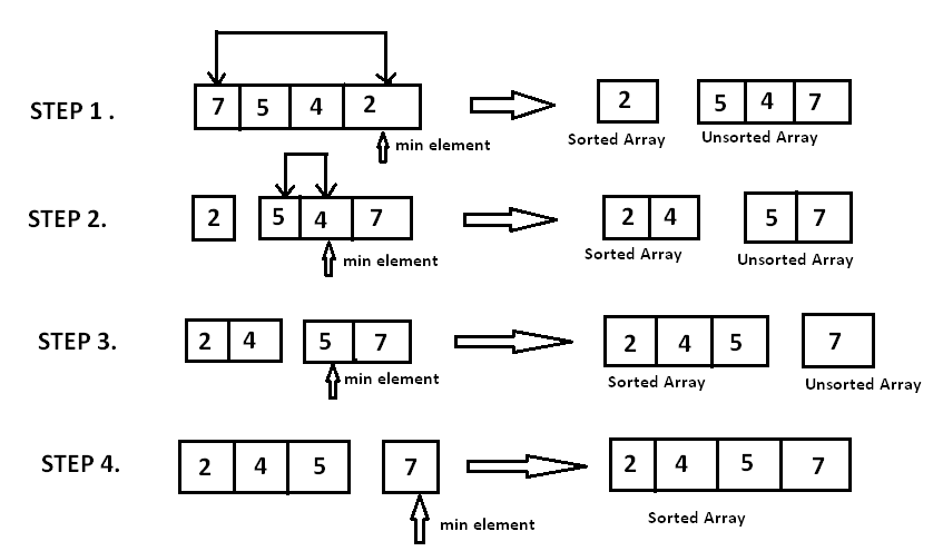
Selection sort

Idea: repeatedly select the smallest (or largest) element from the unsorted portion of the list and move it to the end of the sorted portion of the list
Complexity:
- Time: O($n^2$)
- Space: O($1$)

void selectionSort(int arr[], int n) {
    int i, j, min_idx;

    // One by one move boundary of
    // unsorted subarray
    for (i = 0; i < n - 1; i++) {
        // Find the minimum element in
        // unsorted array
        min_idx = i;
        for (j = i + 1; j < n; j++) {
            if (arr[j] < arr[min_idx])
                min_idx = j;
        }

        // Swap the found minimum element
        // with the first element
        if (min_idx != i)
            swap(arr[min_idx], arr[i]);
    }
}

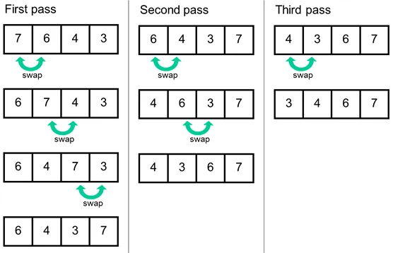
Bubble sort

Idea: repeatedly swap the adjacent elements if they are in the wrong order.
Complexity:
- Time: O($n^2$)
- Space: O($1$)

void bubbleSort(int arr[], int n) {
    int i, j;
    bool swapped;
    for (i = 0; i < n - 1; i++) {
        swapped = false;
        for (j = 0; j < n - i - 1; j++) {
            if (arr[j] > arr[j + 1]) {
                swap(arr[j], arr[j + 1]);
                swapped = true;
            }
        }

        // If no two elements were swapped
        // by inner loop, then break
        if (swapped == false)
            break;
    }
}

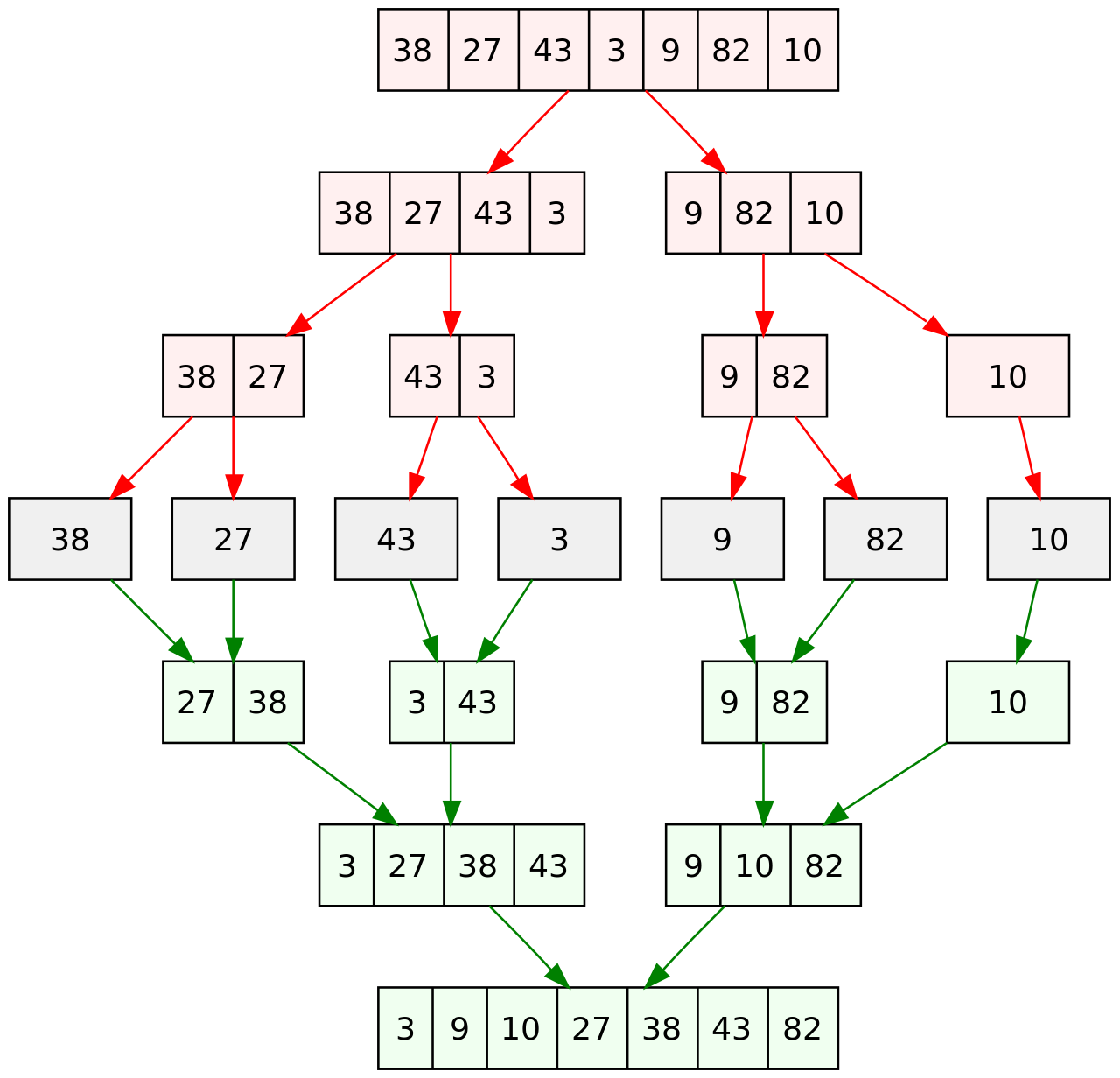
Merge sort

Idea: apply divide and conquer technique by repeatedly dividing the input array into smaller subarrays (halves) and sorting those subarrays then merging them back together to obtain the sorted array
Complexity:
- Time: O($nlog_2(n)$)
- Space: O($n$)

void merge(int arr[], int l, int m, int r) {
  // Create L ← A[l..m] and R ← A[m+1..r]
  int n1 = m - l + 1;
  int n2 = r - m;

  int L[n1], R[n2];

  for (int i = 0; i < n1; i++)
    L[i] = arr[l + i];
  for (int j = 0; j < n2; j++)
    R[j] = arr[m + 1 + j];

  // Maintain current index of sub-arrays and main array
  int i=0, j=0, k=l;

  // Until we reach either end of either L or M, pick larger among
  // elements L and M and place them in the correct position at A[p..r]
  while (i < n1 && j < n2) {
    if (L[i] <= R[j]) {
      arr[k] = L[i];
      i++;
    } else {
      arr[k] = R[j];
      j++;
    }
    k++;
  }

  // When we run out of elements in either L or M,
  // pick up the remaining elements and put in A[p..r]
  while (i < n1) {
    arr[k] = L[i];
    i++;
    k++;
  }

  while (j < n2) {
    arr[k] = R[j];
    j++;
    k++;
  }
}

// Divide the array into two subarrays, sort them and merge them
void mergeSort(int arr[], int l, int r) {
  if (l < r) {
    // m is the point where the array is divided into two subarrays
    int m = l + (r - l) / 2;

    mergeSort(arr, l, m);
    mergeSort(arr, m + 1, r);

    // Merge the sorted subarrays
    merge(arr, l, m, r);
  }
}

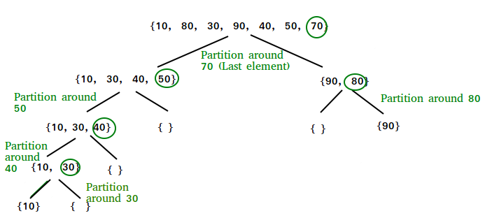
Quick sort

Idea: apply divide and conquer technique by repeatedly picking an elements as a pivot and partitioning the elements around it by comparing it to them
Complexity:
- Time: Θ($nlog_2(n)$), O($n^2$)
- Space: O($1$)

void quickSort(int arr[], int low, int high)
{
    // terminate if range is empty
    if (low >= high)
        return;

    // choose the pivot
    int pivot = arr[high];

    // assume position for the pivot then move it until it reaches the correct sorted position in the array
    int pi = low;

    for (int j = low; j < high; j++) {
        if (arr[j] < pivot) {
            // add the element to the left side and move the pivot forward
            swap(arr[pi], arr[j]);
            pi++;
        }
    }
    swap(arr[pi], arr[high]);

    // repeat for the rest of the array
    quickSort(arr, low, pi - 1);
    quickSort(arr, pi + 1, high);
}

Complexity Comparison summary

Sorting Algorithm	Time Complexity Worst	Time Complexity Average	Time Complexity Best	Space Complexity	Stability
Bubble Sort	O(n^2)	O(n^2)	O(n)	O(1)	Stable
Selection Sort	O(n^2)	O(n^2)	O(n^2)	O(1)	Not Stable
Insertion Sort	O(n^2)	O(n^2)	O(n)	O(1)	Stable
Merge Sort	O(n log n)	O(n log n)	O(n log n)	O(n)	Stable
Quick Sort	O(n^2)	O(n log n)	O(n log n)	O(log n)	Not Stable
Heap Sort	O(n log n)	O(n log n)	O(n log n)	O(1)	Not Stable
Counting Sort	O(n+k)	O(n+k)	O(n+k)	O(k)	Stable
Radix Sort	O(nk)	O(nk)	O(nk)	O(n+k)	Stable

n is the number of elements in the input array.
k is the range of the input (for Counting Sort and Radix Sort).
Stability: A stable sorting algorithm maintains the relative order of records with equal keys.

Labs

Implement Selection sort & Bubble sort & Merge sort on array of integers (3 total)
3011. Find if Array Can Be Sorted
88. Merge Sorted Array
912. Sort an Array
1637. Widest Vertical Area Between Two Points Containing No Points

Two pointers

Idea: works by defining 2 iterators to loop through the data structure, allowing to look at 2 places at the same time
Complexity:
- Time: O($n$)
- Space: O($1$)

bool hasPairSum(vector<int>& arr, int n, int target) {
    // represents first pointer
    int i = 0;

    // represents second pointer
    int j = n - 1;

    while (i < j) {
        // If we find a pair
        if (arr[i] + arr[j] == target)
            return true;

        // If sum of elements at current pointers is less, 
        // we move towards higher values
        else if (arr[i] + arr[j] < target)
            i++;

        // If sum of elements at current pointers is more, 
        // we move towards lower values 
        else
            j--;
    }
    
    return false;
}

Labs

Sliding window

Idea: works by defining 2 iterators to loop through the data structure. allowing to look at the range in between, usual the 2nd iterator adds elements to the range while the 1st removes them
Complexity:
- Time: O($n$)
- Space: O($1$)

int maxSum(int arr[], int n, int k) { // k is window size
    // Compute sum of first window of size k
    int max_sum = 0;
    for (int i = 0; i < k; i++)
        max_sum += arr[i];

    // Compute sums of remaining windows by removing first element of previous
    // window and adding last element of current window.
    int window_sum = max_sum;
    for (int i = k; i < n; i++) {
        window_sum += arr[i] - arr[i - k];
        max_sum = max(max_sum, window_sum);
    }

    return max_sum;
}

Labs

Prefix sum

Idea: cache all previous sums to be able to calculate sum of ranges in O(1)
Complexity:
- Time: O($n$) for build, O(1) for use
- Space: O($n$)

void fillPrefixSum(int arr[], int n) {
    int prefixSum[n];
    prefixSum[0] = arr[0];
    
    // Adding present element with previous element
    for (int i = 1; i < n; i++)
        prefixSum[i] = prefixSum[i - 1] + arr[i];
}

Labs

Frequency array/map

Idea: count the frequency of elements either by using array index or map
Complexity:
- Time: O($n$)
- Space: O($k$), where k is the range of values

void fillFrequencyArray(int arr[], int n, int k) {
    int freq[k] = {0}; // k is 26 for single case alphabet, 58 for both cases
    
    // count elements
    for (int i = 0; i < n; i++)
        freq[arr[i]]++;
}

Labs

Graph

Breadth First Search(BFS)

Idea: iterate through the graph level by level
Usual Complexity:
- Time: O($n$)
- Space: O($m$), where m is max number of elements in a level

void bfs(TreeNode* root) {
	queue<TreeNode*> q;
	q.push(root);
	int lvl = 0;
	
	while (!q.empty()) {
		int c = size(q);
		lvl++;
		
		while (c--) {
			auto cur = q.front();
			q.pop();
			
			if (cur->left)
				q.push(cur->left);
			if (cur->right)
				q.push(cur->right);
				
			cout << cur->val << endl;
		}
	}
}

Labs

Depth First Search(DFS)

Idea: iterate through the graph by visiting the deepest elements first
Usual Complexity:
- Time: O($n$)
- Space: O($d$), where d is max depth of the graph

Iterative:

void dfs(TreeNode* root) {
	stack<TreeNode*> q;
	q.push(root);

	while (!q.empty()) {
		auto cur = q.top();
		q.pop();

		if (cur->left)
			q.push(cur->left);
		if (cur->right)
			q.push(cur->right);

		cout << cur->val << endl;
	}
}

Recursive:

void dfs(TreeNode* node) {
	if(!node) return;

	cout << node->val << endl;

	dfs(node->right), dfs(node->left);
}

Labs

Labs (bonus)

Diameter

Idea: find the distance between the 2 farthest nodes
Complexity:
- Time: O($n$)
- Space: O($n$)
Demo: 3203. Find Minimum Diameter After Merging Two Trees

Using double DFS/BFS

BFS/DFS to find the farthest node from a random node, then another BFS/DFS to find the farthest node from found node and calculate the distance in between

int calcDia(vector<vector<int>>&& adj) {
	int x;
	queue<pair<int, int>> q;

	q.push({0, -1});
	while (!empty(q)) {
		x = q.front().first;

		int c = size(q);
		while (c--) {
			auto [i, p] = q.front();
			q.pop();

			for (auto j : adj[i]) {
				if (j != p)
					q.push({j, i});
			}
		}
	}

	int dia = -1;
	q.push({x, -1});
	while (!empty(q)) {
		dia++;

		int c = size(q);
		while (c--) {
			auto [i, p] = q.front();
			q.pop();

			for (auto j : adj[i]) {
				if (j != p)
					q.push({j, i});
			}
		}
	}

	return dia;
}

Using 1 DFS

The longest diameter has to pass through a node, so maximize on the longest path passing through each node

int f(vector<vector<int>>& adj, int i, int p, int& d) {
	int mx = 0, mx2 = 0;
	for (auto j : adj[i]) {
		if (j == p)
			continue;

		int ret = 1 + f(adj, j, i, d);

		if (ret > mx)
			mx2 = mx, mx = ret;
		else if (ret > mx2)
			mx2 = ret;
	}

	d = max(d, mx + mx2);

	return mx;
}

Backtracking

Idea: try all possible solutions by backtracking steps and retrying
Complexity:
- Time: O($2^n$), or O($n!$)
- Space: O($1$), or O($n$) if keeping track of visits
Demo: 46. Permutations

void permutations(vector<int>& nums, vector<vector<int>>& ans, vector<int> row) {
	if (row.size() == nums.size()) return ans.push_back(row);

	for (int i = 0; i < nums.size(); i++) {
		if (find(begin(row), end(row), nums[i]) == end(row)) {
			row.push_back(nums[i]); // do
			permutations(nums, ans, row);
			row.pop_back(); // undo
		}
	}
}

Floyd-Warshall’s All Pairs Shortest Path

Idea: Relax the graph to find the shortest path between all pairs by trying intermediate steps
Complexity:
- Time: O($n^3$)
- Space: O($n2$) to store results
Demo: 2976. Minimum Cost to Convert String I

void floyd(vector<vector<int>>& minCost) {
	for (size_t k = 0; k < 26; k++) {
		for (size_t i = 0; i < 26; i++) {
			for (size_t j = 0; j < 26; j++) {
				minCost[i][j] = min(minCost[i][j], minCost[i][k] + minCost[k][j]);
			}
		}
	}
}

Dijkstra’s algorithm

Idea: Relax the graph to find the shortest path from 1 node to all others by composing it of other shortest paths (the shortest path contains the shortest intermediate paths)
Complexity:
- Time: O($E*log(V)$), Where E is the number of edges and V is the number of vertices
- Space: O($V$)

void dijkstra(vector<vector<pair<int, int>>> adj, int src){
	int n = size(adj);
	priority_queue<pair<int, int>, vector<pair<int, int>>, greater<pair<int, int>>> pq;
	vector<int> dist(n, INT_MAX);

	// update the source info
	pq.push({ 0, src });
	dist[src] = 0;

	// Loop till empty (no more min dist to relax with)
	while (!empty(pq)) {
		// relax using the min dist
		int i = pq.top().second;
		pq.pop();

		for (auto& [j, w] : adj[i]) {
			// update if this is a better path than the previous
			if (dist[j] > dist[i] + w) {
				dist[j] = dist[i] + w;
				pq.push({ dist[j], j });
			}
		}
	}
}

Labs

1514. Path with Maximum Probability

Dynamic Programing

Idea: like backtracking but with memoization(saving results of visited subsets/states)
Complexity:
- Time: O($n$)
- Space: O($n$)
Demo: 72. Edit Distance

Recursion:

int minDistance(string word1, string word2) {
	const int OO = 1e8;
	int n = size(word1), m = size(word2);
	vector<vector<int>> mem(n, vector<int>(m, -1));
	function<int(int, int)> f = [&](int i, int j) -> int {
		if (i >= n)
			return m - j;
		if (j >= m)
			return n - i;

		if (mem[i][j] != -1)
			return mem[i][j];
		if (word1[i] == word2[j])
			return f(i + 1, j + 1);

		int ret = OO;
		ret = min(ret, 1 + f(i + 1, j));
		ret = min(ret, 1 + f(i, j + 1));
		ret = min(ret, 1 + f(i + 1, j + 1));
		return mem[i][j] = ret;
	};
	return f(0, 0);
}

Tabulation:

int minDistance(string word1, string word2) {
	const int OO = 1e8;
	int n = size(word1), m = size(word2);
	vector<vector<int>> mem(n + 1, vector<int>(m + 1, 0));

	for (size_t i = 0; i < n; i++)
		mem[i][m] = n - i;
	for (size_t j = 0; j < m; j++)
		mem[n][j] = m - j;

	for (int i = n - 1; i >= 0; i--) {
		for (int j = m - 1; j >= 0; j--) {
			int ret = OO;
			if (word1[i] == word2[j])
				ret = min(ret, mem[i + 1][j + 1]);
			else {
				ret = min(ret, 1 + mem[i + 1][j]);
				ret = min(ret, 1 + mem[i][j + 1]);
				ret = min(ret, 1 + mem[i + 1][j + 1]);
			}

			mem[i][j] = ret;
		}
	}

	return mem[0][0];
}

Space optimization:

int minDistance(string word1, string word2) {
	const int OO = 1e8;
	int n = size(word1), m = size(word2);
	vector<vector<int>> mem(2, vector<int>(m + 1, 0));

	bool cur = 0, other = 1;
	for (size_t j = 0; j < m; j++)
		mem[other][j] = m - j;

	for (int i = n - 1; i >= 0; i--) {
		mem[cur][m] = n - i;
		for (int j = m - 1; j >= 0; j--) {
			int ret = OO;
			if (word1[i] == word2[j])
				ret = min(ret, mem[other][j + 1]);
			else {
				ret = min(ret, 1 + mem[other][j]);
				ret = min(ret, 1 + mem[cur][j + 1]);
				ret = min(ret, 1 + mem[other][j + 1]);
			}

			mem[cur][j] = ret;
		}
		other = cur;
		cur = !cur;
	}

	return mem[other][0];
}

Labs

Monotonic Stack

Idea: maintain elements in either increasing or decreasing order to easily find the next greater or smaller element
Complexity:
- Time: O($n$)
- Space: O($n$)
Demo: 1475. Final Prices With a Special Discount in a Shop

vector<int> finalPrices(vector<int>& prices) {
	int n = size(prices);
	stack<int> st;
	for (int i = n - 1; i >= 0; i--) {
		while (!empty(st) && st.top() > prices[i]) {
			st.pop();
		}
		int deal = empty(st) ? 0 : st.top();
		st.push(prices[i]);
		prices[i] -= deal;
	}

	return prices;
}

Labs

KMP Pattern Searching

Idea: efficiently identifies patterns within text by employing a Prefix Table / LPS (Longest Proper Prefix which is also Suffix) Table
Complexity:
- Time: O($n+m$)
- Space: O($m$)
Demo: Print matches’ starting point
Ref: https://www.scaler.in/kmp-algorithm/

string solution(string s, string pattern) {
	int n = size(s), m = size(pattern);

	// lps
	vector<int> lps(m);
	lps[0] = 0;
	int len = 0;
	for (int i = 1; i < m;) {
		if (pattern[i] == pattern[len]) {
			lps[i] = ++len;
			i++;
		} else {
			if (len == 0) {
				lps[i] = 0;
				i++;
			} else {
				len = lps[len - 1];
			}
		}
	}

	// kmp
	int i = 0, j = 0;
	while (i < n) {
		if (s[i] == pattern[j]) {
			i++, j++;
			if (j == m) {
				Printer::print(i - j);
				j = lps[j - 1];
			}
		} else {
			if (j == 0) {
				i++;
			} else {
				j = lps[j - 1];
			}
		}
	}
}

Labs

214. Shortest Palindrome

Data structures

is a systematic way of organizing data for efficient usage.

Main operations:

Random access
Search
Insert
Delete

Each data structure has varying efficiencies with each operation and it’s all about trade-offs so we must carefully select the best candidate for our use case

Array

Concept: a contiguous block of memory is reserved to store blocks of data
Runtime Complexity
- Random access: O(1)
- Search: O(n), (worst case, if target is at the end)
- Insert: O(n), (worst case, if inserting at the beginning or middle, shifting elements is required)
- Delete: O(n), (worst case, if deleting from the beginning or middle, shifting elements is required)

Dynamic Array

Concept: an Array that can be resized, when elements reach a certain usage percent and expands by a certain percent of size
Runtime Complexity
- Random access: O(1)
- Search: O(n), (worst case, if target is at the end)
- Insert: amortized O(1), but O(n) worst case
- Delete: O(n), (worst case, if deleting from the beginning or middle, shifting elements is required)

Labs

LinkedList / Doubly LinkedList

Concept: blocks of data are chained together to form a list
Runtime Complexity
- Random Access: O(n) (sequential access required)
- Search: O(n)
- Insert: O(1) (if inserting at the head or given a reference to a node)
- Delete: O(1) (if given a reference to the node to be deleted)

// Node class
class Node {
public:
    int data;
    Node* prev;
    Node* next;
    Node(int data) : data(data), prev(nullptr), next(nullptr) {}
};

// DoublyLinkedList class
class DoublyLinkedList {
private:
    Node* head;
    Node* tail;

public:
    DoublyLinkedList() : head(nullptr), tail(nullptr) {}

    // Function to get the length of the list
    int getLength() const {
        int length = 0;
        Node* current = head;
        while (current != nullptr) {
            ++length;
            current = current->next;
        }
        return length;
    }

    // Function to insert at the front
    void insertFront(int data) {
        Node* newNode = new Node(data);
        if (head == nullptr) {
            head = tail = newNode;
        } else {
            newNode->next = head;
            head->prev = newNode;
            head = newNode;
        }
    }

    // Function to insert at the back
    void insertBack(int data) {
        Node* newNode = new Node(data);
        if (tail == nullptr) {
            head = tail = newNode;
        } else {
            newNode->prev = tail;
            tail->next = newNode;
            tail = newNode;
        }
    }

    // Function to insert at a specific position
    void insertAtPosition(int data, int position) {
        if (position <= 0) {
            insertFront(data);
            return;
        }
        int length = getLength();
        if (position >= length) {
            insertBack(data);
            return;
        }
        Node* newNode = new Node(data);
        Node* current = head;
        for (int i = 0; i < position - 1; ++i) {
            current = current->next;
        }
        newNode->next = current->next;
        newNode->prev = current;
        if (current->next != nullptr) {
            current->next->prev = newNode;
        }
        current->next = newNode;
    }

    // Function to delete a node with a specific value
    void deleteNode(int data) {
        Node* current = head;
        while (current != nullptr && current->data != data) {
            current = current->next;
        }
        if (current == nullptr) {
            std::cout << "Node with value " << data << " not found." << std::endl;
            return;
        }
        if (current->prev != nullptr) {
            current->prev->next = current->next;
        } else {
            head = current->next;
        }
        if (current->next != nullptr) {
            current->next->prev = current->prev;
        } else {
            tail = current->prev;
        }
        delete current;
    }

    // Function to print the list from front to back
    void printForward() const {
        Node* current = head;
        while (current != nullptr) {
            std::cout << current->data << " ";
            current = current->next;
        }
        std::cout << std::endl;
    }

    // Function to print the list from back to front
    void printBackward() const {
        Node* current = tail;
        while (current != nullptr) {
            std::cout << current->data << " ";
            current = current->prev;
        }
        std::cout << std::endl;
    }

    // Destructor to free memory
    ~DoublyLinkedList() {
        Node* current = head;
        while (current != nullptr) {
            Node* next = current->next;
            delete current;
            current = next;
        }
    }
};

Labs

implement LinkedList on integers
206. Reverse Linked List
876. Middle of the Linked List
1290. Convert Binary Number in a Linked List to Integer

Queue

Concept: you draw the first block of data you insert, first in first out (FIFO)
Runtime Complexity
- Random Access: O(n) (if implemented with a linked list, needs traversal)
- Enqueue: O(1)
- Dequeue: O(1)

// Define the default capacity of a queue
const int MAX_SIZE = 5; // Maximum size of the stack
 
// A class to store a queue
class Queue {
    int *arr;       // array to store queue elements
    int capacity;   // maximum capacity of the queue
    int front;      // front points to the front element in the queue (if any)
    int rear;       // rear points to the last element in the queue
    int count;      // current size of the queue
 
public:
    Queue(int size = MAX_SIZE);     // constructor
    ~Queue();                   // destructor
 
    int dequeue();
    void enqueue(int x);
    int peek();
    int size();
    bool isEmpty();
    bool isFull();
};
 
// Constructor to initialize a queue
Queue::Queue(int size) {
    arr = new int[size];
    capacity = size;
    front = 0;
    rear = -1;
    count = 0;
}
 
// Destructor to free memory allocated to the queue
Queue::~Queue() {
    delete[] arr;
}

 
// Utility function to return the size of the queue
int Queue::size() {
    return count;
}
 
// Utility function to check if the queue is empty or not
bool Queue::isEmpty() {
    return (size() == 0);
}
 
// Utility function to check if the queue is full or not
bool Queue::isFull() {
    return (size() == capacity);
}
 
// Utility function to dequeue the front element
int Queue::dequeue() {
    // check for queue underflow
    if (isEmpty())
    {
        cout << "Underflow\nProgram Terminated\n";
        exit(EXIT_FAILURE);
    }
 
    int x = arr[front];
    cout << "Removing " << x << endl;
 
    front = (front + 1) % capacity;
    count--;
 
    return x;
}
 
// Utility function to add an item to the queue
void Queue::enqueue(int item) {
    // check for queue overflow
    if (isFull())
    {
        cout << "Overflow\nProgram Terminated\n";
        exit(EXIT_FAILURE);
    }
 
    cout << "Inserting " << item << endl;
 
    rear = (rear + 1) % capacity;
    arr[rear] = item;
    count++;
}
 
// Utility function to return the front element of the queue
int Queue::peek() {
    if (isEmpty())
    {
        cout << "Underflow\nProgram Terminated\n";
        exit(EXIT_FAILURE);
    }
    return arr[front];
}

Labs

implement Queue using Array & LinkedList on integers
2073. Time Needed to Buy Tickets
225. Implement Stack using Queues
933. Number of Recent Calls

Stack

Concept: you draw the last block of data you insert, last in first out (LIFO)
Runtime Complexity
- Random Access: O(n) (if implemented with a linked list, needs traversal)
- Push: O(1)
- Pop: O(1)

const int MAX_SIZE = 5; // Maximum size of the stack

class Stack {
private:
    int arr[MAX_SIZE];
    int top;

public:
    Stack() { top = -1;} // Initialize top to -1 to indicate an empty stack

    bool isEmpty() { return (top == -1);}

    bool isFull() { return (top == MAX_SIZE - 1);}

    void push(int element) {
        if (!isFull()) {
            top++;
            arr[top] = element;
            std::cout << "Pushed element: " << element << " onto the stack.\n";
        } else {
            std::cout << "Stack is full. Cannot push element " << element << ".\n";
        }
    }

    void pop() {
        if (!isEmpty()) {
            int poppedElement = arr[top];
            top--;
            std::cout << "Popped element: " << poppedElement << " from the stack.\n";
        } else {
            std::cout << "Stack is empty. Cannot pop from an empty stack.\n";
        }
    }

    int topElement() {
        if (!isEmpty()) {
            return arr[top];
        } else {
            std::cout << "Stack is empty.\n";
            return -1; // In this example, we consider -1 as an invalid value.
        }
    }
};

Labs

implement Stack using Array & LinkedList on integers
20. Valid Parentheses
1021. Remove Outermost Parentheses
1614. Maximum Nesting Depth of the Parentheses

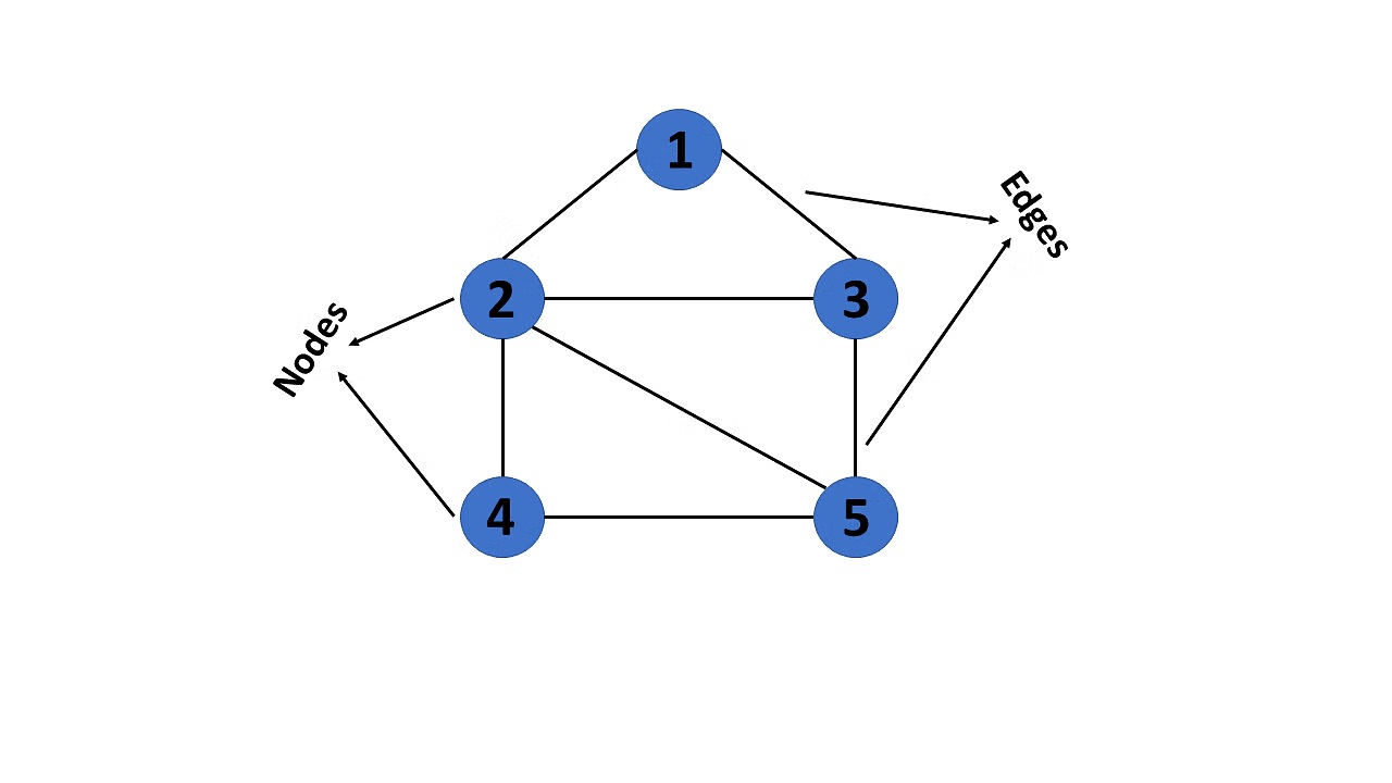
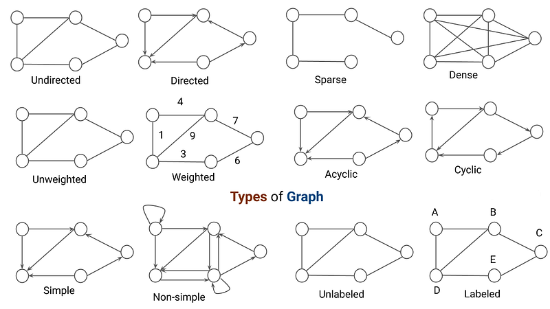
Graph

Concept: blocks of data are called node and the relationships between them are represented by edge connecting 2 nodes
Runtime Complexity
- Random Access: O(n)
- Search: O(n)
- Insert: O(n)
- Delete: O(n)

Terminology:
- Node: basic building block of Graph
- Edge: the linking between 2 nodes
- Path: the sequence of nodes along the edges of a Graph
- Root: a topmost node in a Graph from which edges originate
- Leaf: a node that has no children
- Parent: a predecessor of a node
- Child: a successor of a node
- Sibling: shares the same parent
- Grandparent: parent of parent
- Grandchild: child of child
- Ancestor: parents of parents or parents of parents of parents and so on
- Descendant: children of children or children of children of children and so on
- Degree: number of edges connected to the node
- InDegree: number of edges coming into the node
- OutDegree: number of edges leaving the node
- Isolated node: a Node with a Degree of 0

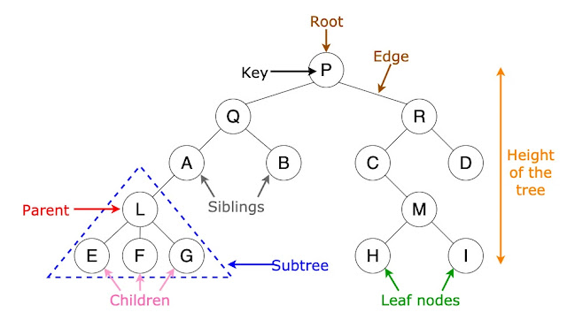
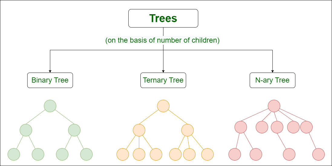
Tree

Concept: is a Directed Acyclic Graph with each node having only 1 parent
Runtime Complexity
- Random Access: O(n)
- Search: O(n)
- Insert: O(n)
- Delete: O(n)
Terminology:
- Root: the topmost node in a Tree
- Height: number of edges on the longest path from the root to a leaf
- Level/Depth: its distance from the root

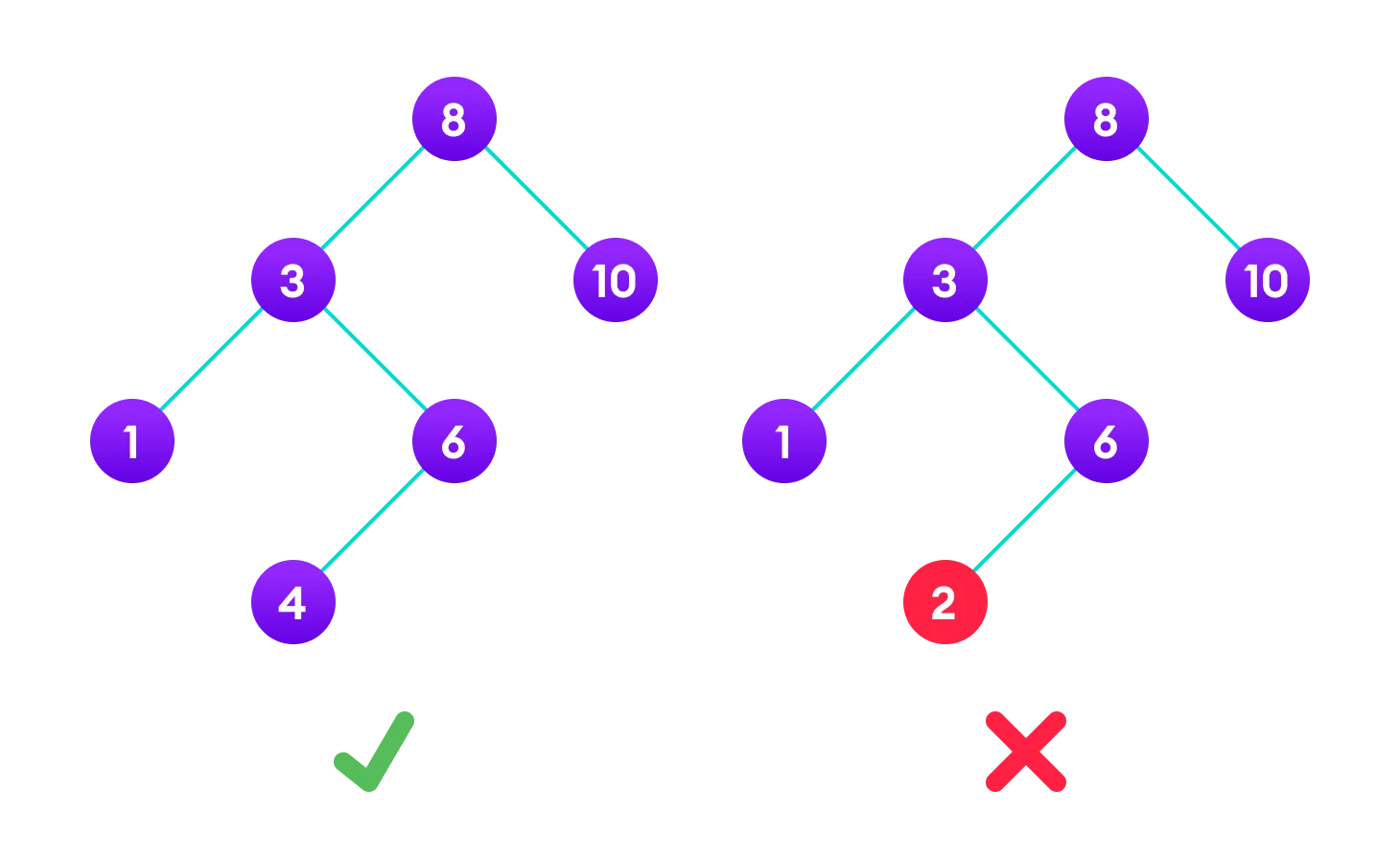
Binary Search Tree

Concept: a binary tree where every node in the left subtree is less than the parent, and every node in the right subtree is of a value greater than the parent
Runtime Complexity
- Random Access: O(log n) average, O(n) worst case (unbalanced tree)
- Search: O(log n) average, O(n) worst case (unbalanced tree)
- Insert: O(log n) average, O(n) worst case (unbalanced tree)
- Delete: O(log n) average, O(n) worst case (unbalanced tree)

Labs

Set

Concept: stores unique blocks of data
Type:
- HashSet: unsorted set (fastest)
- TreeSet: sorted set

HashSet

Concept: A Set built using a hash table to store and retrieve data by hash
Runtime Complexity
- Random Access: Not supported. HashSet does not maintain any order of elements, and it does not provide a method to access elements by index.
- Search: O(1) average, O(n) worst-case due to hash collisions.
- Insert: O(1) average, O(n) worst-case due to hash collisions.
- Delete: O(1) average, O(n) worst-case due to hash collisions.

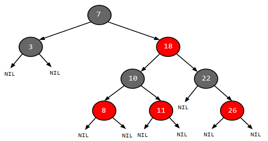
TreeSet

Concept: a Set where data is sorted (built based on a Red-Black tree)
Runtime Complexity
- Random Access: Not supported. TreeSet does not maintain an index-based structure.
- Search: O(log n)
- Insert: O(log n)
- Delete: O(log n)

Labs

Map

Concept: stores data in pairs of key & value, with key being unique and the value representing a block of data
Type:
- HashMap: unsorted map (fastest)
- TreeMap: sorted map

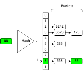
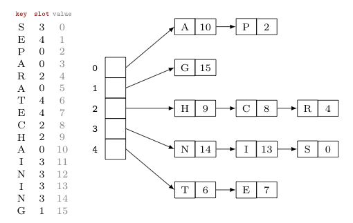
HashMap

Concept: a Map built using a hash table to store and retrieve keys by hash
Runtime Complexity
- Random Access: O(1) average, O(n) worst case (if many collisions)
- Search: O(1) average, O(n) worst case (if many collisions)
- Insert: O(1) average, O(n) worst case (if resizing is required)
- Delete: O(1) average, O(n) worst case (if many collisions)

TreeMap

Concept: a Map where keys are sorted (built based on a Red-Black tree)
Runtime Complexity
- Random Access: Not supported. TreeMap does not maintain an index-based structure.
- Search: O(log n)
- Insert: O(log n)
- Delete: O(log n)

Labs

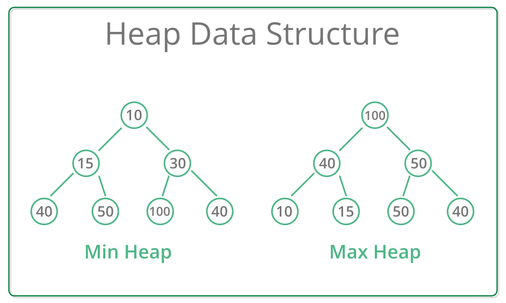
Heap / Priority Queue

Concept: a Balanced binary tree where for every node the values of its children is less than or equal to its own value, (can also customize this comparison)
Runtime Complexity
- Random Access (find min/max): O(1)
- Search: O(n)
- Insert: O(log n)
- Delete: O(log n) (removing the root and reheapifying)

Labs

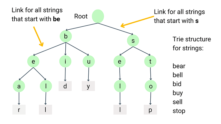
Prefix Tree (Trie)

Concept: a Tree for storing and retrieving strings efficiently by connecting letters in chains
Runtime Complexity
- Random Access: Not applicable. Tries are not designed for direct index-based access to elements.
- Search: O(m), where m is the length of the string being searched.
- Insert: O(m), where m is the length of the string being inserted.
- Delete: O(m), where m is the length of the string being deleted.

Labs

Complexity Comparison summary

Data Structure	Random Access	Search	Insert	Delete
Array	O(1)	O(n)	O(n)	O(n)
Linked List	O(n)	O(n)	O(1)	O(1)
Queue	O(n)	O(n)	O(1)	O(1)
Stack	O(n)	O(n)	O(1)	O(1)
BST	O(log n)*	O(log n)*	O(log n)*	O(log n)*
HashSet	Not supported	O(1)**	O(1)**	O(1)**
TreeSet	Not supported	O(log n)	O(log n)	O(log n)
HashMap	O(1)**	O(1)**	O(1)**	O(1)**
TreeMap	Not supported	O(log n)	O(log n)	O(log n)
Heap	O(1)	O(n)	O(log n)	O(log n)

* BST complexities are average cases; worst-case scenarios (unbalanced) are O(n)
** HashSet and HashMap complexities are average cases; worst-case scenarios with many collisions are O(n)